Note
Click here to download the full example code
Use of Multi-Fidelity Kriging
from smt.applications import MFK,NestedLHS
import numpy as np
import otsmt
import matplotlib.pyplot as plt
import openturns as ot
Definition of Initial data
# Construction of the DOE
# low fidelity model
def lf_function(x):

    return (
        0.5 * ((x * 6 - 2) ** 2) * np.sin((x * 6 - 2) * 2)
        + (x - 0.5) * 10.0
        - 5
    )

# high fidelity model
def hf_function(x):

    return ((x * 6 - 2) ** 2) * np.sin((x * 6 - 2) * 2)

# Problem set up
xlimits = np.array([[0.0, 1.0]])
xdoes = NestedLHS(nlevel=2, xlimits=xlimits, random_state=0)
xt_c, xt_e = xdoes(4)

# Evaluate the HF and LF functions
yt_e = hf_function(xt_e)
yt_c = lf_function(xt_c)

xv_e = np.linspace(xlimits[0][0],xlimits[0][1],50)[:,np.newaxis]
yv_e  = hf_function(xv_e)
Out:
/usr/share/miniconda3/envs/test/lib/python3.9/site-packages/numpy/lib/function_base.py:2845: RuntimeWarning: Degrees of freedom <= 0 for slice
  c = cov(x, y, rowvar, dtype=dtype)
/usr/share/miniconda3/envs/test/lib/python3.9/site-packages/numpy/lib/function_base.py:2704: RuntimeWarning: divide by zero encountered in divide
  c *= np.true_divide(1, fact)
/usr/share/miniconda3/envs/test/lib/python3.9/site-packages/numpy/lib/function_base.py:2704: RuntimeWarning: invalid value encountered in multiply
  c *= np.true_divide(1, fact)
Training of smt model for Multi-Fidelity Kriging
sm_mfk = MFK(theta0=xt_e.shape[1] * [1.0])

# low-fidelity dataset names being integers from 0 to level-1
sm_mfk.set_training_values(xt_c, yt_c, name=0)
# high-fidelity dataset without name
sm_mfk.set_training_values(xt_e, yt_e)

# train the model
sm_mfk.train()
Out:
___________________________________________________________________________

                                    MFK
___________________________________________________________________________

 Problem size

      # training points.        : 4

___________________________________________________________________________

 Training

   Training ...
   Training - done. Time (sec):  0.0519252
Creation of OpenTurns PythonFunction for prediction
otmfk = otsmt.smt2ot(sm_mfk)
otmfkprediction = otmfk.getPredictionFunction()
otmfkpvariances = otmfk.getConditionalVarianceFunction()
otmfkgradient = otmfk.getPredictionDerivativesFunction()
print('Predicted values by MFK:',otmfkprediction(xv_e))
print('Predicted variances values by MFK:',otmfkpvariances(xv_e))
print('Prediction derivatives by MFK:',otmfkgradient(xv_e))
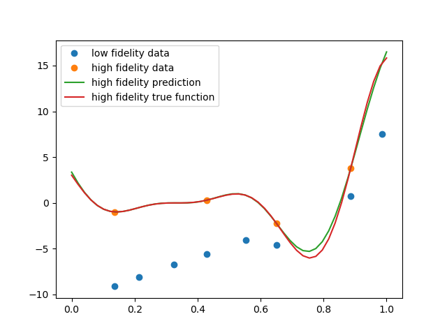
plt.figure()
plt.plot(xt_c,yt_c,'o',label='low fidelity data')
plt.plot(xt_e,yt_e,'o',label='high fidelity data')
plt.plot(xv_e,otmfkprediction(xv_e),label='high fidelity prediction')
plt.plot(xv_e,yv_e,label='high fidelity true function')
plt.legend()
Out:
___________________________________________________________________________

 Evaluation

      # eval points. : 50

   Predicting ...
   Predicting - done. Time (sec):  0.0003684

   Prediction time/pt. (sec) :  0.0000074

Predicted values by MFK:      [ y0           ]
 0 : [  3.36259     ]
 1 : [  2.17245     ]
 2 : [  1.15711     ]
 3 : [  0.33716     ]
 4 : [ -0.278041    ]
 5 : [ -0.691552    ]
 6 : [ -0.918828    ]
 7 : [ -0.986409    ]
 8 : [ -0.929369    ]
 9 : [ -0.787746    ]
10 : [ -0.602325    ]
11 : [ -0.410289    ]
12 : [ -0.241288    ]
13 : [ -0.114471    ]
14 : [ -0.0369421   ]
15 : [ -0.00389078  ]
16 : [ -0.000468516 ]
17 : [ -0.00519364  ]
18 : [  0.00554832  ]
19 : [  0.0525371   ]
20 : [  0.149013    ]
21 : [  0.296968    ]
22 : [  0.485052    ]
23 : [  0.68852     ]
24 : [  0.871351    ]
25 : [  0.990384    ]
26 : [  1.001       ]
27 : [  0.863646    ]
28 : [  0.550373    ]
29 : [  0.0504842   ]
30 : [ -0.62548     ]
31 : [ -1.44402     ]
32 : [ -2.34954     ]
33 : [ -3.2678      ]
34 : [ -4.1116      ]
35 : [ -4.78823     ]
36 : [ -5.20775     ]
37 : [ -5.29133     ]
38 : [ -4.97881     ]
39 : [ -4.23458     ]
40 : [ -3.05145     ]
41 : [ -1.45195     ]
42 : [  0.51281     ]
43 : [  2.7666      ]
44 : [  5.2135      ]
45 : [  7.74458     ]
46 : [ 10.2454      ]
47 : [ 12.6034      ]
48 : [ 14.715       ]
49 : [ 16.4913      ]
Predicted variances values by MFK:      [ y0           ]
 0 : [ 10.179       ]
 1 : [  5.4472      ]
 2 : [  2.59355     ]
 3 : [  1.05755     ]
 4 : [  0.344588    ]
 5 : [  0.0767776   ]
 6 : [  0.0067112   ]
 7 : [  0.000419647 ]
 8 : [  0.00301542  ]
 9 : [  0.00213815  ]
10 : [  0.000283986 ]
11 : [  0.000237495 ]
12 : [  0.00148185  ]
13 : [  0.00216881  ]
14 : [  0.00155617  ]
15 : [  0.000452678 ]
16 : [  1.84457e-06 ]
17 : [  0.000446884 ]
18 : [  0.00105183  ]
19 : [  0.00102818  ]
20 : [  0.000409195 ]
21 : [  2.54515e-07 ]
22 : [  0.000496539 ]
23 : [  0.00167399  ]
24 : [  0.00249858  ]
25 : [  0.00212468  ]
26 : [  0.000850067 ]
27 : [  7.85821e-06 ]
28 : [  0.000686052 ]
29 : [  0.00237432  ]
30 : [  0.00307325  ]
31 : [  0.00147847  ]
32 : [  4.55678e-05 ]
33 : [  0.00638104  ]
34 : [  0.0307624   ]
35 : [  0.0798767   ]
36 : [  0.149854    ]
37 : [  0.223325    ]
38 : [  0.274021    ]
39 : [  0.278435    ]
40 : [  0.229328    ]
41 : [  0.143252    ]
42 : [  0.0559062   ]
43 : [  0.00506563  ]
44 : [  0.00840297  ]
45 : [  0.0489685   ]
46 : [  0.0809975   ]
47 : [  0.0621786   ]
48 : [  0.00761714  ]
49 : [  0.0498522   ]
___________________________________________________________________________

 Evaluation

      # eval points. : 50

   Predicting ...
   Predicting - done. Time (sec):  0.0003324

   Prediction time/pt. (sec) :  0.0000066

Prediction derivatives by MFK:      [ y0          ]
 0 : [ -62.1445    ]
 1 : [ -54.2438    ]
 2 : [ -45.0897    ]
 3 : [ -35.1879    ]
 4 : [ -25.1268    ]
 5 : [ -15.5246    ]
 6 : [  -6.96728   ]
 7 : [   0.0549673 ]
 8 : [   5.20445   ]
 9 : [   8.33791   ]
10 : [   9.52639   ]
11 : [   9.0485    ]
12 : [   7.35596   ]
13 : [   5.01416   ]
14 : [   2.62452   ]
15 : [   0.738605  ]
16 : [  -0.22404   ]
17 : [  -0.0420272 ]
18 : [   1.26837   ]
19 : [   3.44776   ]
20 : [   6.02491   ]
21 : [   8.38203   ]
22 : [   9.84636   ]
23 : [   9.79587   ]
24 : [   7.76439   ]
25 : [   3.53107   ]
26 : [  -2.81922   ]
27 : [ -10.8744    ]
28 : [ -19.917     ]
29 : [ -28.9875    ]
30 : [ -36.9827    ]
31 : [ -42.7774    ]
32 : [ -45.3526    ]
33 : [ -43.9181    ]
34 : [ -38.0104    ]
35 : [ -27.558     ]
36 : [ -12.9048    ]
37 : [   5.20984   ]
38 : [  25.7114    ]
39 : [  47.2828    ]
40 : [  68.4792    ]
41 : [  87.8517    ]
42 : [ 104.067     ]
43 : [ 116.015     ]
44 : [ 122.885     ]
45 : [ 124.22      ]
46 : [ 119.935     ]
47 : [ 110.3       ]
48 : [  95.9066    ]
49 : [  77.5972    ]
___________________________________________________________________________

 Evaluation

      # eval points. : 50

   Predicting ...
   Predicting - done. Time (sec):  0.0003662

   Prediction time/pt. (sec) :  0.0000073


<matplotlib.legend.Legend object at 0x7f1210b7ff40>
Total running time of the script: ( 0 minutes 0.193 seconds)