Principle of AK methods
The reliability problem to solve is: \(P_f = \mathbb{P}[g\left( \mathbf{X},\mathbf{d} \right) \leq T)]\)
\(\mathbf{X}\) is the input random vector of dimension \(n\), \(f_\mathbf{X}(\mathbf{x})\) its joint density probability function. \(\mathbf{d}\) is a deterministic vector, \(g(\mathbf{X},\mathbf{d})\) is the limit state function of the model. \(D_f = \{\mathbf{X} \in \mathbb{R}^n \, \vert \, g(\mathbf{X},\mathbf{d}) \leq T\}\) is the domain definition of the event to consider (failure). \(g(\cdot) = 0\) is called the limit state.
The failure condition can also be \(g(\mathbf{X},\mathbf{d})\geq T\).
The probability of failure can be defined as follows : \(P_f = \mathbb{P}[g(\mathbf{X},\mathbf{d})\leq T]= \int_{D_f} f_\mathbf{X}(\mathbf{x}) d\mathbf{x}\)
This probability can also be written as : \(P_f = \int_{\mathbb{R}^n} \mathbf{1}_{ \left\{ g(\mathbf{X},\mathbf{d}) \leq T \right\} }f_\mathbf{X}(\mathbf{x}) d\mathbf{x}\)
In case of rare event probability estimation, the surrogate model has to be accurate in the zones that are relevant to the failure probability estimation i.e. in the vicinity of failure threshold \(T\) and in the high probability content regions. The use of the exact function \(g\) and its surrogate \(\hat{g}\) in the probability calculation will lead to the same result if \(\forall \mathbf{x} \in \mathbb{R}^d, \mathbf{1}_{g(\mathbf{x})<T} = \mathbf{1}_{\hat{g}(\mathbf{x})<T}\) with \(\hat{g}\) the surrogate model of \(g\).
In case of rare event probability estimation, the surrogate model has to be accurate in the zones that are relevant to the failure probability estimation i.e. in the vicinity of failure threshold \(T\) and in the high probability content regions.
Active-learning methods consist (AK-MCS, AK-IS, AK-SS, etc.) in refining only the samples (generated by the reliability method) that are uncertain with respect the threshold exceedance in order to limit the uncertainty provided by the metamodel to the failure probability. The goal is to minimize the number of samples that have to be evaluated on the real function in the probability simulation.**
From the initial training set \(\mathcal{X}\), the Gaussian process properties (i.e. estimation of the predicted error variance) are valuable to determine the additional samples which have to be evaluated on $g(cdot)$ to refine its surrogate model. Different refinement strategies have been developed in the litterature.
Active-learning techniques generally use the following scheme :
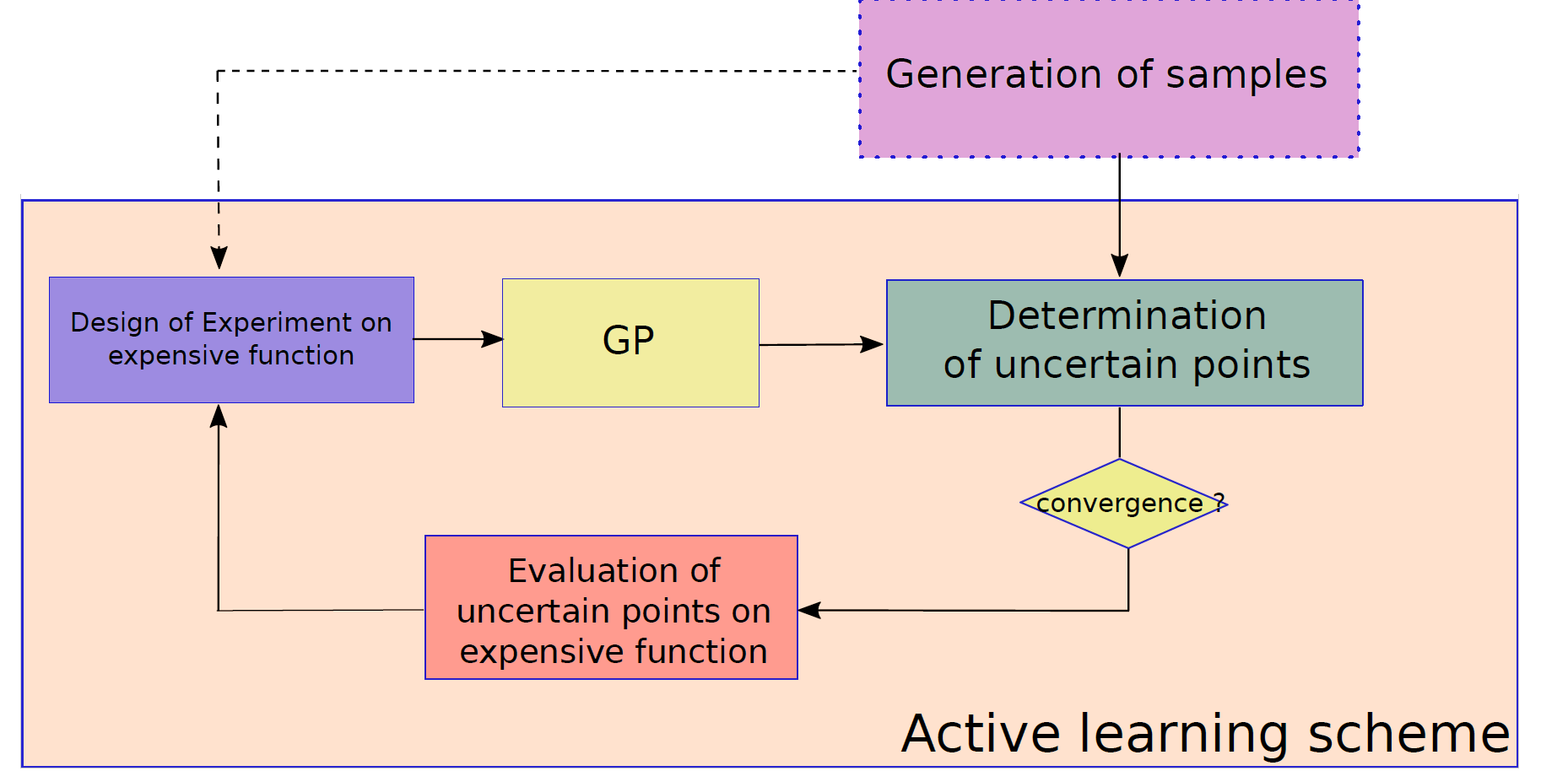
From the initial training set \(\mathcal{X}\), the Gaussian process properties (i.e. estimation of the predicted error variance) are valuable to determine the additional samples which have to be evaluated on \(\phi(\cdot)\) to refine its surrogate model. Different refinement strategies have been developed in the literature. Here, the method described in [Echard 2011] is implemented ("U criterion").
This method determines a new sample point \(\mathbf{x}\) to add to the training set \(\mathcal{X}\) by solving the following optimisation problem: \(\underset{\mathbf{x}}{\max} \left[1 - \Phi_{0,1}\left( \frac{\left|T-\hat{g}(\mathbf{x},\mathcal{X})\right|}{\hat{\sigma}(\mathbf{x},\mathcal{X})} \right)\right]\)
where \(\Phi_{0,1}(\cdot)\) is the cdf of the standard Gaussian distribution, \(\hat{\phi}\) the mean prediction of the Kriging and \(\hat{\sigma}\) the estimated standard deviation of the prediction error.
The used criterion generates a sample for which the Kriging prediction is closed to the threshold (numerator) and which presents a high prediction error (denominator). Due to the monotonicity of the involved cdf, the optimisation problem is equivalent to:
\(\underset{\mathbf{x}}{\min}\; \frac{\left|T-\hat{g}(\mathbf{x},\mathcal{X})\right|}{\hat{\sigma}(\mathbf{x},\mathcal{X})}\)
This criterion has been coupled with usual reliability methods present in OpenTURNS. In practice, the optimisation problem is not solved, and given a sample set \(\{\mathbf{X}_1,\dots, \mathbf{X}_N\}\) provided by the reliability algorithm the new sample which will be added to the training set is determined by
\(\mathbf{X} = \underset{\mathbf{X}_1,\dots,\mathbf{X}_N}{\text{argmin}} \left\{\frac{\left|T-\hat{g}(\mathbf{X}_1,\mathcal{X})\right|}{\hat{\sigma}(\mathbf{X}_1,\mathcal{X})},\dots, \frac{\left|T-\hat{g}(\mathbf{X}_N,\mathcal{X})\right|}{\hat{\sigma}(\mathbf{X}_N,\mathcal{X})} \right\}\)
References
Echard, B., Gayton, N., & Lemaire, M. (2011). AK-MCS: an active learning reliability method combining Kriging and Monte Carlo simulation. Structural Safety, 33(2), 145-154.
Echard, B. (2012). Assessment by kriging of the reliability of structures subjected to fatigue stress, Université Blaise Pascal, PhD thesis
Huan (2016). Assessing small failure probabilities by AK–SS: An active learning method combining Kriging and Subset Simulation, Structural Safety 59 (2016) 86–95